모두의 연구소에서 진행하는
"함께 콘텐츠를 제작하는 콘텐츠 크리에이터 모임"
COCRE(코크리) 1기 회원으로 제작한 글입니다.
코크리란? 🐘
들어가며
모델링은 중요합니다. 하지만 그 모델을 잘 만든 후에 학습을 시키는 것도 중요합니다. 모델을 만들고 fit()해서 쉽게 학습하는 것은 편하지만 작은 것들 하나하나 컨트롤해보기 어렵고 혹은 문제가 생겼을 때 디버깅해보기 불편합니다. 저는 예전 version의 tensorflow와 input 모양이 바뀌어서 고생을 한 적이 있습니다. 백퍼 fit의 input 모양 때문인지는 확실하진 않아요 ㅎ.. fit()을 사용하는 대신 직접 모델을 학습하는 트레이너를 만들어 모델을 학습해봅시다!
저는 model.fit()에서 벗어나고 싶은 사람, tfds.load(’mnist’)로 mnist 데이터 말고 새로운 데이터 혹은 커스텀 데이터를 쓰는 튜토리얼을 읽고 싶은 사람, 커스텀 데이터를 model.fit()으로 학습하는 방법 말고 커스텀 트레이너로 학습하고 싶은 사람들을 위한 글을 쓰고 싶었습니다.
⚠️ 주의 : 포켓몬 트레이너와는 다릅니다.

제가 처음 딥러닝을 하던 때에 각종 멋진 딥러닝 Github들의 Directory Tree가 멋지다고 생각했습니다. 그것들은 너무나 알맞게 잘 구성되어 있었죠. 우리도 잠깐 우리의 작은 프로젝트가 어떨지 생각해보며, Directory Tree를 구성해보고 시작하는건 어떨까요?
/Users/eden/ByeModelFitFunc
├── dataset
│   ├── adho mukha svanasana
│   ├── bhujangasana
│   ├── ...
│   └── yoganidrasana
├── dataset.py				# dataset loader
├── label.txt				# dataset 클래스 이름이 있는 txt 파일
├── loss.py				# loss function
├── main.py				# model and data set, train
├── trainer.py				# trainer
└── model.py				# model
우리의 프로젝트는 위와 같이 구성될 것입니다. 늘어날지도 모르지만요. 늘어나려나? 모르겠어요.
데이터 로드하기
딥러닝 모델을 학습할 때는 무엇이 필요할까요? 데이터, 모델, loss 함수, optimizer 정도가 필요할 것 같아요. 우리는 모델을 학습하기 이전에 먼저 데이터를 가져와야 합니다. 이전에 Keras의 ImageDataGenerator를 사용하여 손쉽게 로드해왔으리라 생각됩니다. ImageDataGenerator는 아주 손쉽게 원하는 배치 사이즈만큼 이미지도 불러올 수 있고, 이미지 사이즈도 바꿀 수 있습니다. 하지만 우리는 잠시 ImageDataGenerator를 내려놓고 tf.data로 데이터를 가져오는 방법을 사용할 것입니다. tf.data를 사용하면 좋은 점은 Tensorflow 피셜 큰 사이즈의 데이터를 로드하기가 아주 좋으며, 재사용 가능한 조각들로 복잡한 입력 파이프라인을 구축할 수 있다는 것이라고 합니다. 제가 tf.data를 사용하게 된 이유는 큰 사이즈 데이터를 로드하기에 좋다는 것이었습니다.
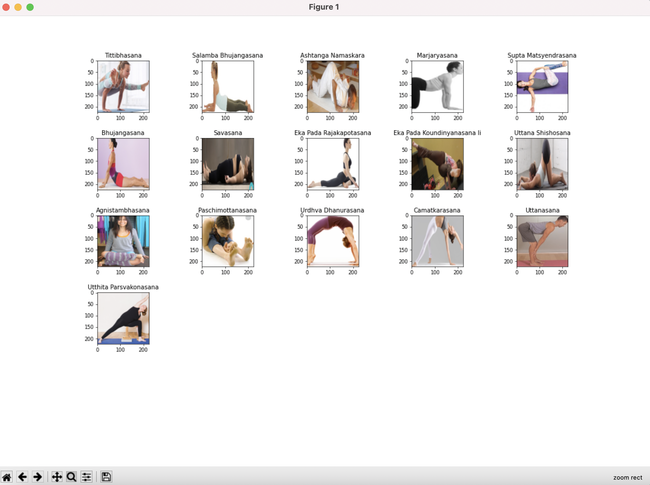
그전에, 잠시 이 작은 프로젝트에서 사용할 데이터를 소개합니다. 우리는 Kaggle의 Yoga Pose Image classification dataset을 사용할 예정이고, 총 107개의 요가 동작과 그에 따른 이미지들이 있습니다. 저도 한 번도 사용해본 적 없는 데이터라서 과연 분류가 잘될지 궁금하네요 😁
데이터 로드, 모델 학습 과정을 모두 저와 같은 데이터로 테스트해보고 싶으시다면 아래의 링크를 따라서 다운로드하여보세요!
https://www.kaggle.com/shrutisaxena/yoga-pose-image-classification-dataset
Yoga Pose Image classification dataset
image dataset for yoga pose estimation
www.kaggle.com
자 아래와 같이 tf.data를 이용해서 데이터를 가져오도록 하였습니다.
import os
import pathlib
import numpy as np
import tensorflow as tf
import matplotlib.pyplot as plt


def get_label(file_path, class_names):
    parts = tf.strings.split(file_path, os.path.sep)
    return parts[-2] == class_names


def process_path(file_path, class_names, img_shape=(224, 224)):
    label = tf.strings.split(file_path, os.path.sep)
    label = label[-2] == class_names

    img = tf.io.read_file(file_path)
    img = tf.image.decode_jpeg(img, channels=3)
    img = tf.image.convert_image_dtype(img, tf.float32)
    img = tf.image.resize(img, img_shape)
    return img, label


def prepare_for_training(ds, batch_size=32, cache=True, shuffle_buffer_size=1000):
    if cache:
        if isinstance(cache, str):
            ds = ds.cache(cache)
        else:
            ds = ds.cache()

    ds = ds.shuffle(buffer_size=shuffle_buffer_size)
    ds = ds.repeat()
    ds = ds.batch(batch_size)
    ds = ds.prefetch(buffer_size=tf.data.experimental.AUTOTUNE)

    return ds


def load_label(label_path):
    class_names = []
    with open(label_path) as f:
        for line in f:
            line = line.strip()
            class_names.append(line)

    return np.array(class_names)


def show_batch(image_batch, label_batch, class_names):
    size = len(image_batch)
    sub_size = int(size ** 0.5) + 1

    plt.figure(figsize=(10, 10), dpi=80)
    for n in range(size):
        plt.subplot(sub_size, sub_size, n+1)
        plt.subplots_adjust(left=0.125, bottom=0.1, right=0.9, top=0.9, wspace=0.2, hspace=0.5)
        plt.title(class_names[label_batch[n]==True][0].title())
        plt.imshow(image_batch[n])
    plt.show()


def load_data(data_path, label_path, batch=32):
    class_names = load_label(label_path)
    data_dir = pathlib.Path(data_path)
    list_ds = tf.data.Dataset.list_files(str(data_dir / '*/*'))

	# 데이터 확인
    # for f in list_ds.take(5):
    #     print(f.numpy())

    labeled_ds = list_ds.map(lambda x: process_path(x, class_names))
    train_ds = prepare_for_training(labeled_ds, batch_size=batch)

    return train_ds
dataset.py에 작성되어 있는 코드로 만든 train_dataset 로더가 이미지와 라벨을 잘 가져오는지 확인해봅시다.
for img, label in train_dataset.take(1):
    show_batch(img, label, class_names)
아래의 이미지를 보세요. 요가 동작의 이름은 너무 어렵지만 잘 가져오는 것 같습니다.
위의 코드에서 간단히 코드의 역할들을 몇 가지를 짚어보고 갑시다. 아래 설명 혹은 tensorflow docs를 참고해도 좋습니다.
1) tf.data.Dataset.list_files
출력 결과를 참고해보면 data_dir의 하위의 모든 파일들을 가져오는 역할을 한다는 것을 알 수 있습니다.
data_dir = './dataset'
list_ds = tf.data.Dataset.list_files(str(data_dir / '*/*'))

for f in list_ds.take(5):
	print(f.numpy())

## 출력 결과
b'dataset/eka pada rajakapotasana/21-0.png'
b'dataset/astavakrasana/11-0.png'
b'dataset/halasana/39-1.png'
b'dataset/matsyasana/20-0.png'
b'dataset/bhujangasana/17-0.png'
2) list_ds.map(lambda x: process_path(x, class_names))
데이터셋에 변환(transformation)을 적용할 때 사용할 수 있습니다. 코드에서는 process_path라는 함수로 변환을 적용하게 만들었는데 라벨과 이미지에 대한 변환을 적용했다는 것을 알 수 있습니다. resize 외에도 다양한 augmentation 코드를 추가해볼 수 있을 것입니다!
def process_path(file_path, class_names, img_shape=(224, 224)):
    label = tf.strings.split(file_path, os.path.sep)	# file path parse해서 라벨 얻기
    label = label[-2] == class_names	# 라벨 인코딩

    img = tf.io.read_file(file_path)	# 이미지 읽기
    img = tf.image.decode_jpeg(img, channels=3)	# 이미지 파일 디코딩
    img = tf.image.convert_image_dtype(img, tf.float32)	# 이미지 타입 변환
    img = tf.image.resize(img, img_shape)	# 이미지 사이즈 변환
    return img, label

labeled_ds = list_ds.map(lambda x: process_path(x, class_names))
3) cache(), shuffle(), repeat(), batch(), prefetch() 함수
아래의 설명이 어렵다면 여기를 참고하셔도 좋습니다. 이 글이 가장 설명을 잘했다고 생각합니다. 아래에 제 설명과 함께 글을 번역하여 추가했습니다.
- ds.cache() : 데이터셋을 메모리에 저장해 두고, 두 번째 이터레이션부터는 캐시 된 데이터를 사용하여 시간을 아낄 수 있습니다. Epoch 동안 실행되는 일부 작업(예: 파일 열기 및 데이터 읽기)이 저장됩니다.
- ds.shuffle(buffer_size=shuffle_buffer_size) : 데이터셋을 섞어(shuffle) 줍니다. BUFFER_SIZE 만큼 임의로 샘플을 뽑고, 뽑은 샘플은 다른 샘플로 대체합니다. 완벽한 셔플링을 위해서는 데이터셋의 전체 크기보다 크거나 같은 버퍼 크기가 필요합니다.
내가 가진 데이터 셋 : [1, 2, 3, 4, 5, 6]
dataset.shuffle(buffer_size=3)은 버퍼 사이즈 3만큼 랜덤 하게 뽑습니다. 이렇게 생각하면 됩니다 :
랜덤 버퍼
   |
   |   다른 모든 데이터들이 있는 있는 소스 데이터 셋
   |         |
   ↓         ↓
[1,2,3] <= [4,5,6]
2가 랜덤 버퍼에서 나갔다고 생각해봅시다. 그럼 한 자리 빈 버퍼는 소스 데이터 셋에서 채워집니다. 그게 바로 4가 될 거예요:
2 <= [1,3,4] <= [5,6]
아무것도 남지 않을 때까지 계속 반복한다면? :
1 <= [3,4,5] <= [6] 5 <= [3,4,6] <= [] 3 <= [4,6] <= [] 6 <= [4] <= [] 4 <= [] <= []
- ds.repeat() : 데이터셋을 반복하여 생성합니다. repeat안에 반복하고 싶은 수를 넣어주지 않으면 무한히 반복합니다.
- ds.batch(batch_size) : batch_size 만큼의 배치로 알아서 묶어줍니다. ds.repeat()는 ds.batch() 호출 이전에 있어야 합니다. 그래야 계속 데이터가 생성되기 때문입니다.
- ds.prefetch(buffer_size=tf.data.experimental.AUTOTUNE) : 학습 중일 때, 데이터 로드 시간을 줄이기 위해 미리 메모리에 적재시켜 둡니다. 즉, 모델이 step s를 실행하는 동안 입력 파이프라인은 step s+1의 데이터를 미리 읽습니다. 대부분의 dataset input 파이프라인은 prefetch 호출로 끝나야 합니다.
def prepare_for_training(ds, batch_size=32, cache=True, shuffle_buffer_size=1000, n_repeat=3):
    if cache:
        if isinstance(cache, str):
            ds = ds.cache(cache)
        else:
            ds = ds.cache()

    ds = ds.shuffle(buffer_size=shuffle_buffer_size)
    ds = ds.repeat(n_repeat)
    ds = ds.batch(batch_size)
    ds = ds.prefetch(buffer_size=tf.data.experimental.AUTOTUNE)

    return ds
모델 만들기
자 이제 데이터를 가져오도록 파이프라인을 만들었으니, 모델을 구성해보도록 합시다. 우리는 efficientnetb0를 가져와서 사용할 것입니다! 케라스가 백본을 지원해줍니다. 편-안
import tensorflow as tf
from tensorflow.keras.applications import EfficientNetB0

class YogaPose(tf.keras.Model):
    def __init__(self, num_classes=30, freeze=False):
        super(YogaPose, self).__init__()
        self.base_model = EfficientNetB0(include_top=False, weights='imagenet')

        # Freeze the pretrained weights
        if freeze:
            self.base_model.trainable = False

        self.top = tf.keras.Sequential([tf.keras.layers.GlobalAveragePooling2D(name="avg_pool"),
                                       tf.keras.layers.BatchNormalization(),
                                       tf.keras.layers.Dropout(0.5, name="top_dropout")])
        self.classifier = tf.keras.layers.Dense(num_classes, activation="softmax", name="pred")

    def call(self, inputs, training=True):
        x = self.base_model(inputs)
        x = self.top(x)
        x = self.classifier(x)
        return x


if __name__ == '__main__':
    model = YogaPose(num_classes=107, freeze=True)
    model.build(input_shape=(None, 224, 224, 3))
    print(model.summary())
위와 같이 model.py에 YogaPose라는 이름을 가진 모델을 이렇게 만들었습니다. 유의할 점은 제가 만든 모델은 base model인 EfficientNetB0를 freeze 시키고 싶은지 아닌지를 결정해서 학습해야 된다는 것입니다.
트레이너 만들기
우리는 이제 데이터도 있고 모델도 가지고 있습니다. 이제 학습만 하면 됩니다. Tensorflow docs를 참고하여 만들었습니다.
import tensorflow as tf
from model import YogaPose
from dataset import load_data


class Trainer:
    def __init__(self, model, epochs, batch, loss_fn, optimizer):
        self.model = model
        self.epochs = epochs
        self.batch = batch
        self.loss_fn = loss_fn

    def train(self, train_dataset, train_metric):
        for epoch in range(self.epochs):
            print("\nStart of epoch %d" % (epoch,))
            # Iterate over the batches of the dataset.
            for step, (x_batch_train, y_batch_train) in enumerate(train_dataset):
                with tf.GradientTape() as tape:
                    logits = model(x_batch_train, training=True)
                    loss_value = self.loss_fn(y_batch_train, logits)
                    # tf.print(loss_value)
                grads = tape.gradient(loss_value, model.trainable_weights)
                self.optimizer.apply_gradients(zip(grads, model.trainable_weights))

                # Update training metric.
                train_metric.update_state(y_batch_train, logits)

                # Log every 5 batches.
                if step % 5 == 0:
                    print(
                        "Training loss (for one batch) at step %d: %.4f"
                        % (step, float(loss_value))
                    )
                    print("Seen so far: %d samples" % ((step + 1) * self.batch))
                    print(train_metric.result().numpy())

                # Display metrics at the end of each epoch.
            train_acc = train_acc_metric.result()
            print("Training acc over epoch: %.4f" % (float(train_acc),))
loss function, optimizer를 모두 train()의 매개변수로 넣어주었지만 생성자에 같이 넣는 게 더 좋을지도 모르겠습니다. 코드를 잠깐 뜯어봅시다.
train 함수는 아래 코드와 같이 시작합니다. 왜죠? 원하는 epoch 만큼 학습을 해야하기 때문입니다. 매 epoch 마다 print 문을 찍어뒀습니다. 그리고 매 배치를 가져올 때마다 with tf.GradientTape() as tape라는 것 안에 들어갑니다. 이건 뭘까요? 테이프..? 웬 테이프..
for epoch in range(self.epochs):
    print("\nStart of epoch %d" % (epoch,))
    # Iterate over the batches of the dataset.
    for step, (x_batch_train, y_batch_train) in enumerate(train_dataset):
        with tf.GradientTape() as tape:
딥러닝을 학습이라는 것은 모델이 loss 혹은 cost라고 불리우는 이 값을 최소화시키도록 만든다는 것이라고 할 수 있습니다. 이 과정에서 backpropagation을 합니다. 초심으로 돌아가서 다시 본다면 아래 이미지가 설명하는 바로 그것이었습니다.
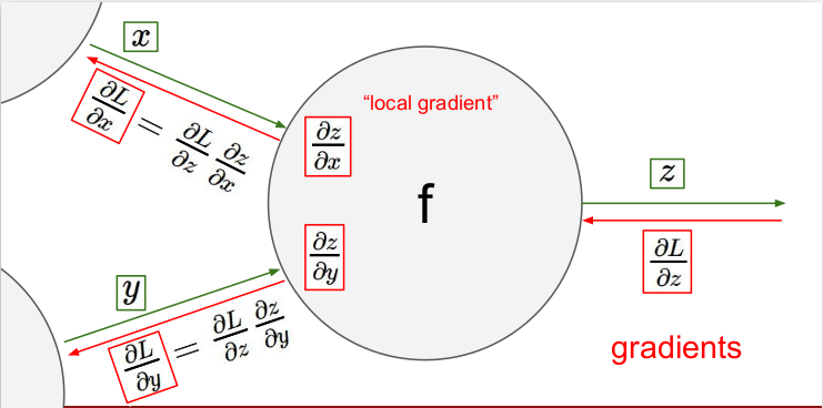
Tensorflow docs에서 이렇게 설명해줍니다. tf.GradientTape는 컨텍스트(context) 안에서 실행된 모든 연산을 테이프(tape)에 "기록"합니다. 그 다음 텐서플로는 후진 방식 자동 미분(reverse mode differentiation)을 사용해 테이프에 "기록된" 연산의 그래디언트를 계산합니다. 말로만 설명하면 어렵기 때문에 예시를 하나 가져왔습니다.
x가 3.0이라는 스칼라 값을 가지고 있는 변수이고 $y=x^2$ 이라는 함수라고 할 때 GradientTape.gradient(target, sources)를 사용하여 그라디언트를 구한다고 한다면 아래와 같은 값을 얻을 수 있습니다.
x = tf.Variable(3.0)

with tf.GradientTape() as tape:
  y = x**2

# dy = 2x * dx
dy_dx = tape.gradient(y, x)
dy_dx.numpy()

# 출력 결과
6.0
그렇기 때문에 우리는 tf.GradientTape를 사용합니다.
모델이 예측한 값은 logit이 될 것입니다. 그리고 로스 함수로부터 true label과 모델이 예측한 logits 사이의 loss를 구할 수 있겠습니다. 후에 tape.gradient()로 그라디언트를 계산하고 optimizer에 적용시켜줍니다. 마지막으로 train metric.update_state는 각 배치마다 모델을 평가하는 metric에 알맞은 값을 업데이트해줍니다.
	logits = model(x_batch_train, training=True)
	loss_value = loss_fn(y_batch_train, logits)
    # tf.print(loss_value)
grads = tape.gradient(loss_value, model.trainable_weights)
optimizer.apply_gradients(zip(grads, model.trainable_weights))

# Update training metric.
train_metric.update_state(y_batch_train, logits)
이제 학습이 되는지 확인해볼까요!
loss function, optimizer는 물론 커스텀으로도 가능하지만 이번엔 그냥 있는 걸 가져다 쓰려고 합니다. 아마도 귀찮아서 그런 것이 아니라 🤭 이다음 튜토리얼에서 Trainer에 progbar와 같은 기능들을 추가해보고 커스텀 로스도 사용해보겠습니다. 그리고 저는 3배 치마다 train_metric.result()를 출력하도록 하였습니다.
epoch = 1
batch = 32

model = YogaPose(num_classes=107)
dataset, DATASET_SIZE = load_data(data_path='./dataset', label_path='./label.txt')

loss_function = tf.keras.losses.CategoricalCrossentropy()
# loss_function = CustomAccuracy()
optimizer = tf.keras.optimizers.Adam()
train_acc_metric = tf.keras.metrics.CategoricalAccuracy()

trainer = Trainer(model=model,
                  epochs=epoch,
                  batch=batch)
trainer.train(train_dataset=dataset,
              loss_fn=loss_function,
              optimizer=optimizer,
              train_metric=train_acc_metric)
자 학습이 과연 잘 될까요? 노트북으로 학습하며.. 일할 때 회사 멀티 GPU로 학습을 핑핑 돌리는 게 얼마나 행운이었는지를 깨닫습니다. loss가 아주 잘 줄고 있네요.
## 학습 출력 결과의 일부

Start of epoch 0
Training loss (for one batch) at step 0: 6.2404
Seen so far: 32 samples
0.0
Training loss (for one batch) at step 3: 2.0699
Seen so far: 128 samples
0.15625
Training loss (for one batch) at step 6: 1.0305
Seen so far: 224 samples
0.4017857
Training loss (for one batch) at step 9: 0.3091
Seen so far: 320 samples
0.5625
Training loss (for one batch) at step 12: 0.0147
Seen so far: 416 samples
0.65865386
Training loss (for one batch) at step 15: 0.0129
Seen so far: 512 samples
0.72265625
Training loss (for one batch) at step 18: 0.1871
Seen so far: 608 samples
0.7615132
Training loss (for one batch) at step 21: 0.0032
Seen so far: 704 samples
0.79403406
Training loss (for one batch) at step 24: 0.0025
Seen so far: 800 samples
0.81875
Training loss (for one batch) at step 27: 0.0003
Seen so far: 896 samples
0.83816963
Training loss (for one batch) at step 30: 0.0023
Seen so far: 992 samples
0.85383064
하지만 학습만 한다고 끝은 아니겠죠. 모델도 저장해야 되고, 데이터가 작을 땐 몰라도 크면 얼마나 배치가 돌아가고 있는지 궁금합니다. 그렇기 때문에 ProgBar도 있으면 좋겠죠. 모델을 저장할 때도 모든 모델을 저장하는 것은 이미 로컬에 이 데이터 저 데이터 저장해둬서 고통받고 있는 컴퓨터에게 무리한 요구일 수 있습니다. 가장 좋은 모델을 저장하는 것도 괜찮은 방법일 것 같습니다.
이 글에서는 tf.data를 사용하여 데이터를 로드하고, 트레이너를 만들어 단순히 학습하는 것까지 진행해보았습니다. 바로 위에서 이야기한 모든 기능들은 다음 편에서 진행해보겠습니다. 그리고 다음에는 모델을 저장하고 요가 자세 모델이 얼마나 완벽한지 테스트해봅시다.

다음 편도 읽어주실 거죠? 핳

안오신다고요? 못들은척 하겠습니다
끝
'DL|ML' 카테고리의 다른 글
| Foursquare - Location Matching 컴피티션 캐글 노트북 번역 (0) | 2022.05.07 |
|---|---|
| model.fit()에서 벗어나기! (2) (0) | 2022.04.20 |
| Mapping Africa’s Buildings with Satellite Imagery (0) | 2021.12.10 |
| <혼자 또는 같이하는 머신러닝 스터디 잼> 티셔츠 대장정의 끝 (0) | 2021.05.20 |
| 정확히 CNN에서 shared weights란 무엇을 의미하나요? (0) | 2021.05.12 |


