[Tübingen ML] Computer Vision - Lecture 2.1 (Image Formation: Primitives and Transformations)

 

튀빙겐 대학교의 Lecture: Computer Vision 2.1을 공부하며 정리한 자료입니다.

 

Lecture 2.1 (Image Formation: Primitives and Transformations)

 

 

Primitives and Transformations

• Geometric primitives는 3D shapes를 묘사하기 위한 basic building blocks이고, 여기서는 points, lines, planes(점, 선 면) 을 이야기한다.
• Basic transformation에 대해 이야기한다.

 

2D Points

2D points는 각각 inhomogeneous coordinates, homogeneous 좌표로 아래와 같이 쓸 수 있다.

[그림 1] 2D points inhomogeneous coordinates

[그림 2] 2D points homogeneous coordinates

 

• $l : (a, b, c)$라는 직선이 있을 때 $(a, b, c)$는 직선 $l$을 유일하게 표현하지 않는다. $(ka, kb, kc)$와 같이 상수 $k$를 곱해서 동일한 직선 $l$을 표현할 수 있다.
• 이러한 관계에 있는 모든 벡터들을 동치관계(equivalent)에 있다고 하고 이 벡터들을 homogeneous 벡터라고 한다.
• $\mathbb{R}^3$공간에서 동치관계에 있는 모든 벡터들의 집합을 사영공간(projective space) $\mathbb{P}^2$라고 한다.

 

[그림 3]

[그림 3]처럼 inhomogeneous 벡터인 $\mathtt{x}$에 1을 추가하면 homogeneous 벡터로 바꿀 수 있다.

[그림 4]

 

homogeneous points의 $\tilde{w} = 0$일 때 ideal points 혹은 points at infinity라고 부른다.

[그림 5]

 

---

2D Lines

평면의 한 점은 행벡터 $(x, y)$가 아닌 열벡터 $(x, y)^\intercal$로 표시한다.

2D lines은 homogeneous coordinates $\tilde{l} = (a, b, c)^\intercal$를 사용하여 나타낼 수 있다 :

 

[그림 6]

normalize $\tilde{l}$를 $\tilde{l} = (n_x, n_y, d)^{\intercal} = (\mathtt{n}, d)^{\intercal} $ with $ ||n||_2 =1$이라고 표현할 수 있다. 이 때 $\mathtt{n}$은 line에 수직인 법선 벡터이고 $d$는 origin으로부터의 거리이다. 

 

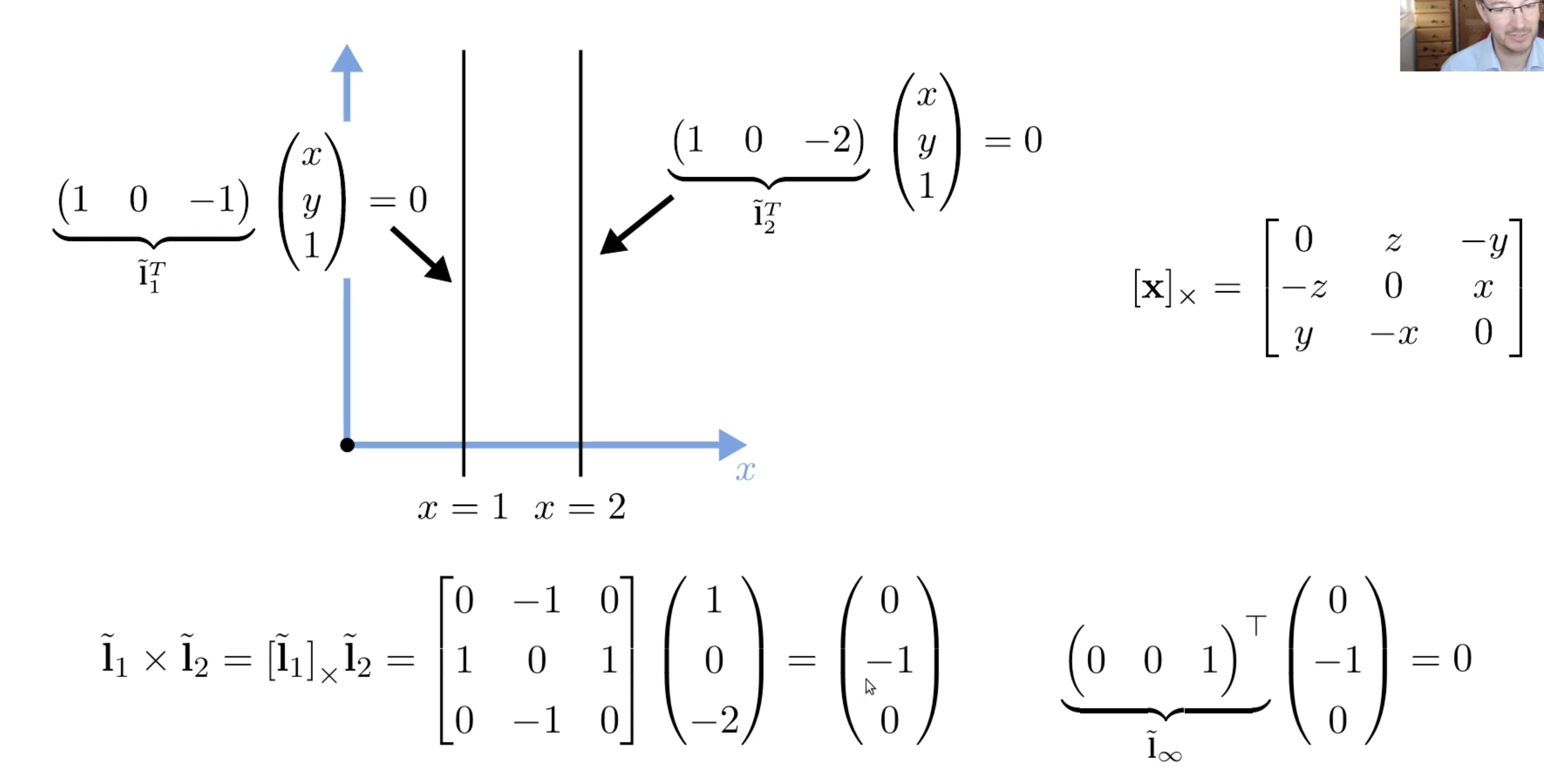
Cross Product

Cross product(벡터곱)은 아래와 같이 표현할 수 있다.

[그림 7]

 

 

2D Line Arithmetic

Homogeneous coordinates에서 두 lines의 intersection(교점)은 $\tilde{x} = \tilde{l}_1 \times \tilde{l}_2$이고, 두 점들을 지나는 직선(line joining two points)은 $\tilde{l} = \overline{\mathtt{x}}_1 \times \overline{\mathtt{x}}_2$로 나타낼 수 있다.

 

[그림 8] 교점 구하는 예

 

[그림 9] 교점 구하는 예 2 : 평행하는 직선

 

2D Conics

[그림 10]

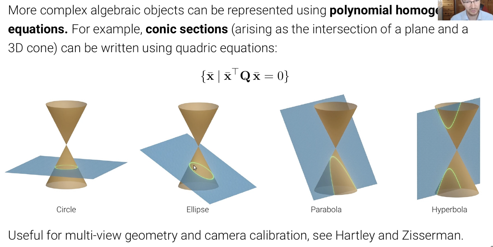
이 강의에서는 자세히 다루지 않는다.

 

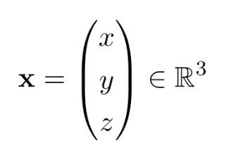
3D Points

3D points는 inhomogeneous coordinates로 [그림 11] 처럼 쓸 수 있다.

[그림 11]

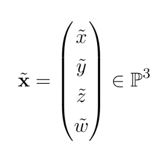
homogeneous coordinates로는 [그림 12]처럼 쓸 수 있다. 2D랑 비슷함.

[그림 12]

 

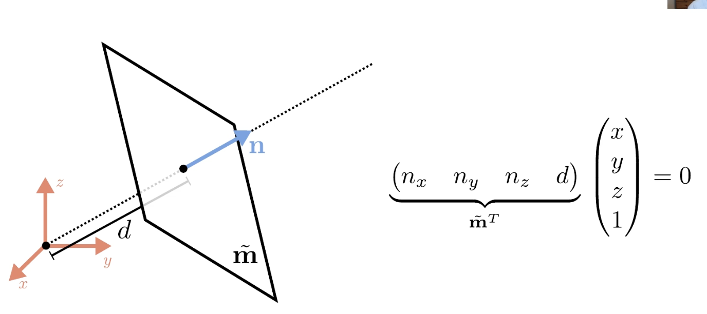
3D Planes

3D planes는 homogeneous coordinates $\tilde{m} = (a, b, c, d)^\intercal$으로 표현할 수 있다.

[그림 13]

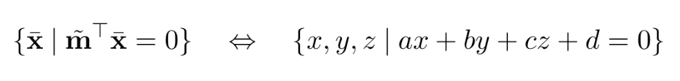
normalize $\tilde{m}$를 $\tilde{m} = (n_x, n_y, n_z, d)^{\intercal} = (\mathtt{n}, d)^{\intercal} $ with $ ||n||_2 =1$이라고 표현할 수 있다. 이 때 $\mathtt{n}$은 plane에 수직인 법선 벡터이고 $d$는 origin으로부터의 거리이다. 

[그림 14]

 

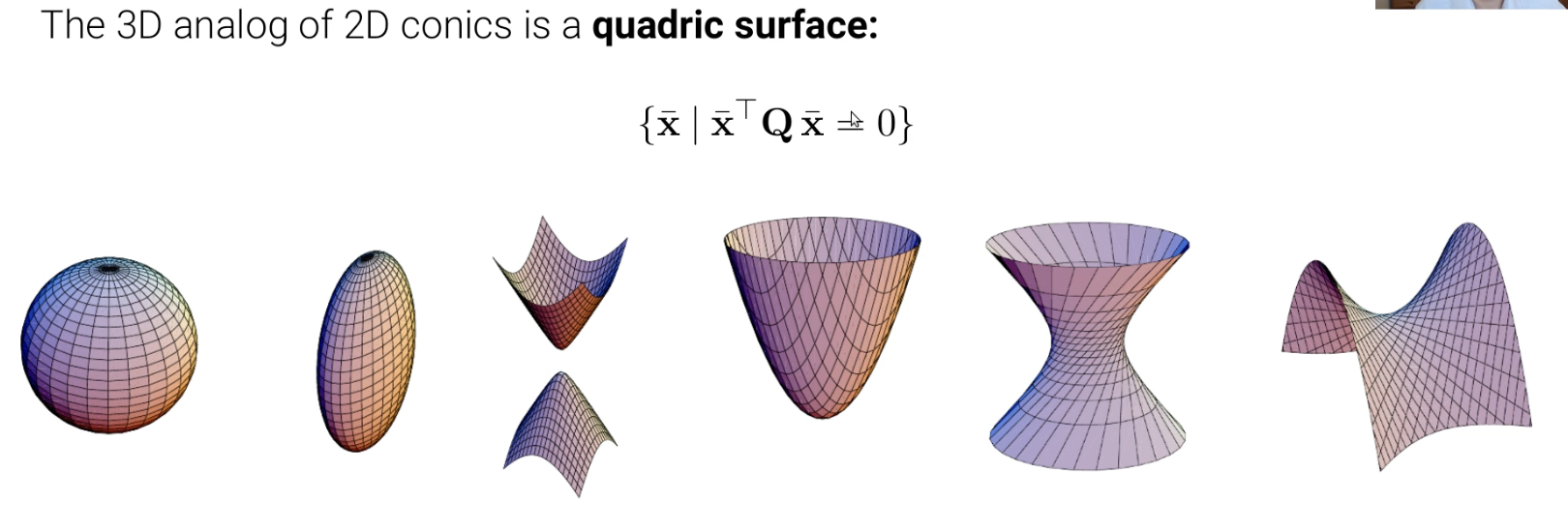
3D Quadrics

Q에 따라 모양이 바뀐다.

[그림 15]

 

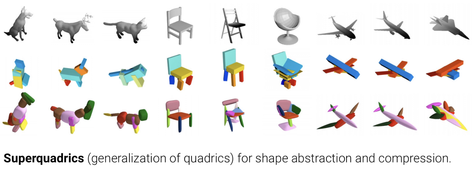
[그림 16]은 해당 강의의 교수님이 연구한 논문인데 Superquadics라고 한다. 대충 듣고 이해한바로는 quadric의 일반화 버전이고 objects의 shape을 콤팩트하게 표현할 수 있는 거라고 한다. 

 

[그림 16] Superquadics

 

 

2D Transformations

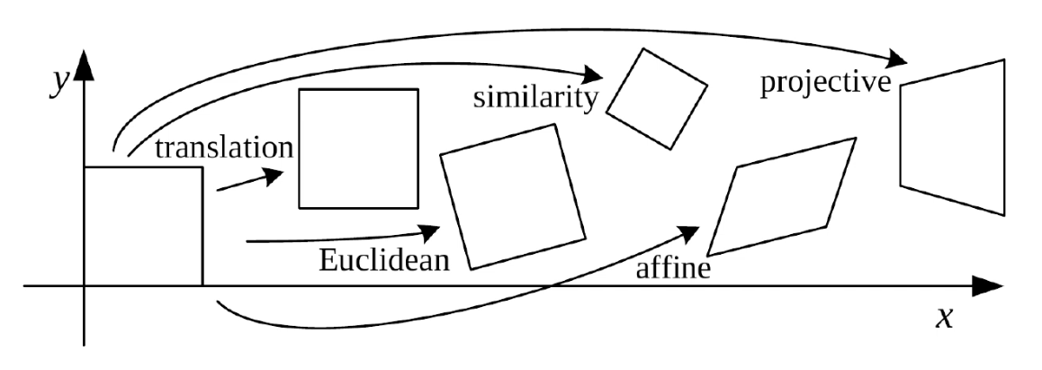
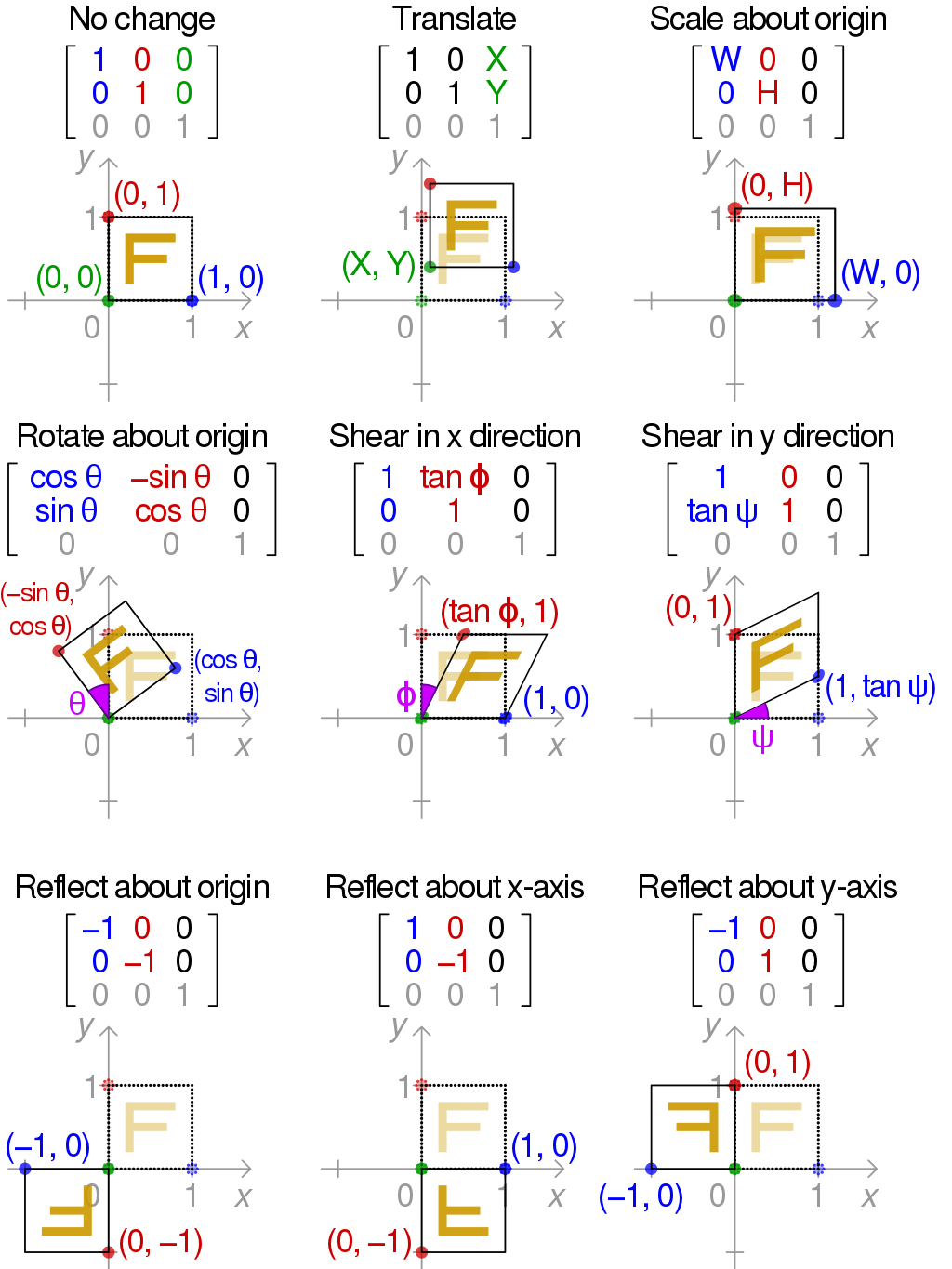
[그림 17] 2D Transformations

Translation

[그림 18] Translations transformation

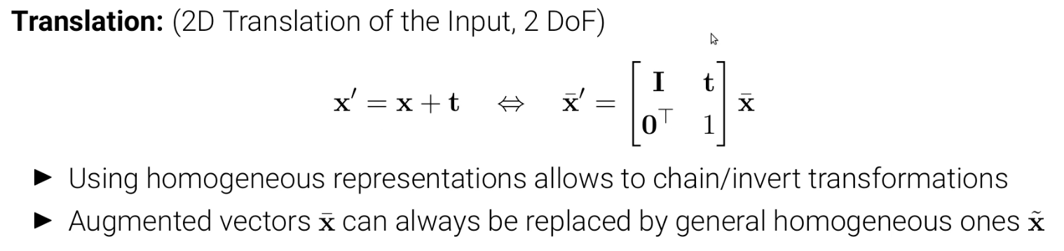
• Homogeneous representations은 transformation의 chain/invert를 가능하게 한다.

 

Euclidean

[그림 19] Euclidean, isometry transformation

 

[그림 20] 위키피디아 - Transformation matrix

 

• $\begin{pmatrix} x' \\ y' \\ 1 \end{pmatrix} = \begin{bmatrix} \epsilon cos\theta & -sin\theta & t_x \\ \epsilon \sin\theta & cos\theta & t_y \\ 0 & 0 & 1 \end{bmatrix} \begin{pmatrix} x \\ y \\ 1 \end{pmatrix}$ 로 나타낼 수 있다. $\epsilon = \pm{1}$이고 $\epsilon = +1$이면 방향을 유지하고, $\epsilon = -1$이면 방향을 바꾼다.
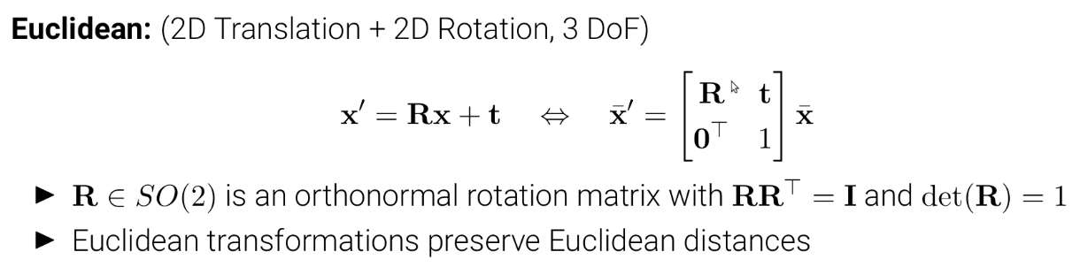
• 또 다른 말로는 isometry 한국어로는 등거리 사상이라고 한다.
• 물체가 변환 전과 후 크기가 동일할 때를 isometry 변환이라고 한다.
• I는 $2 \times 2$ 회전 행렬이고 t는 2차원 이동 벡터이다.
• 자유도가 3이다. 회전이 1(아마도 세타..?), 이동이 2($t_x$, $t_y$ 인듯)

 

Similarity

[그림 21] similarity transformation

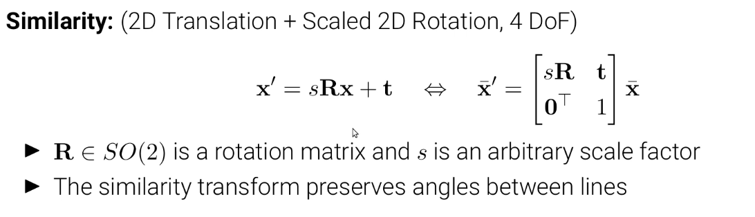
• Euclidean 변환과 배율(scaling) 조정의 합성 변환이다.
• $\begin{pmatrix} x' \\ y' \\ 1 \end{pmatrix} = \begin{bmatrix} s cos\theta & -s sin\theta & t_x \\ s \sin\theta & s cos\theta & t_y \\ 0 & 0 & 1 \end{bmatrix} \begin{pmatrix} x \\ y \\ 1 \end{pmatrix}$ 로 나타낼 수 있다. s는 스칼라이고 배율 조정을 나타낸다.
• Euclidean transformation에 배율 조정인 s를 추가한 자유도 4를 가진다.

 

Affine

[그림 22] Affine transformation

 

• $\begin{pmatrix} x' \\ y' \\ 1 \end{pmatrix} = \begin{bmatrix} a_{11} & a_{12} & t_x \\ a_{21} & a_{22} & t_y \\ 0 & 0 & 1 \end{bmatrix} \begin{pmatrix} x \\ y \\ 1 \end{pmatrix}$ 로 나타낼 수 있다.
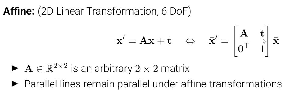
• 6 자유도를 가진다.
• 평행한 직선을 보전하는 성질을 가진다.

 

Perpective

[그림 23] perspective transformation

• $x' = \mathtt{H}_{\mathtt{p}} \mathtt{x} = \begin{bmatrix} A & t \\ v^\intercal & \upsilon \end{bmatrix} \mathtt{x}$로 나타낼 수 있다. $ v = (\upsilon_1, \upsilon_2)^\intercal$는 벡터다. 행렬 $A$는 affine 변환에서 나온다.
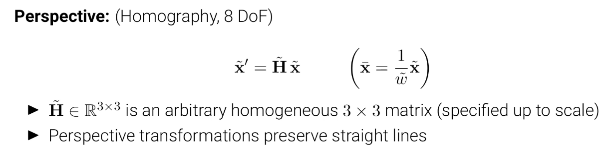
• 8 자유도를 가진다.
• Projective transformation은 다른 transformation들로 분해가 가능하다. $\mathtt{H}_p = \mathtt{H}_S \mathtt{H}_A \mathtt{H}_P$

 

Overview of 2D Transformations

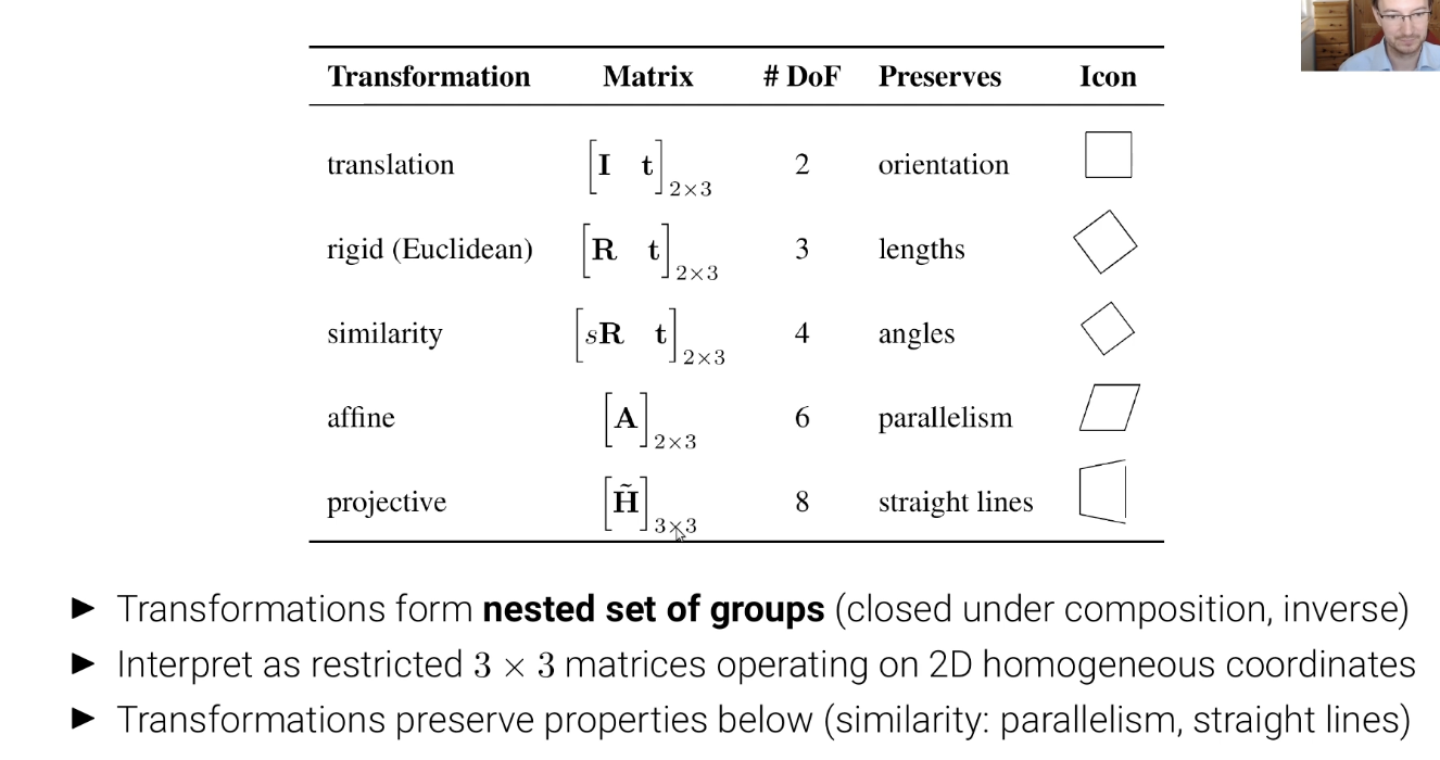
[그림 24] overview of 2D transformations

 

 

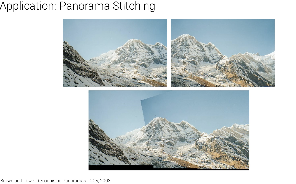
Application: Panorama Stitching

Transformation으로 파노라마를 만들 수 있음. 왼쪽 오른쪽 이미지를 맞추기 위해 이동, 회전, 스케일 조정 등을 해야하기 때문에 transformation이 사용됨.

[그림 24] 파노라마

 

 

Reference

• 튀빙겐 대학교 computer vision lecture
• Multiple View Geometry in Computer Vision(컴퓨터 비전을 위한 다중 시점 기하학)
• Multiple View Geometry 책 내용 정리 파트1